Regression R-Squared

Hi,

again I have a really very special topic. I am currently doing some quant work and work with regression analysis.

Optuma have some great tools and functions about regression analysis but I have still some questions about how to work with these regression tools and functions.

I used the tool “Correlation” to calculate the correlation between Apple and the S&P 500. I created TWO examples, one chart using “% change” in the setting “Calculate on” and another chart using “Price” in the setting “Calculate on”.

correl#1

correl#2

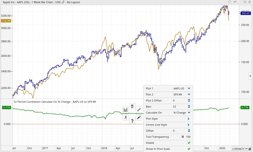
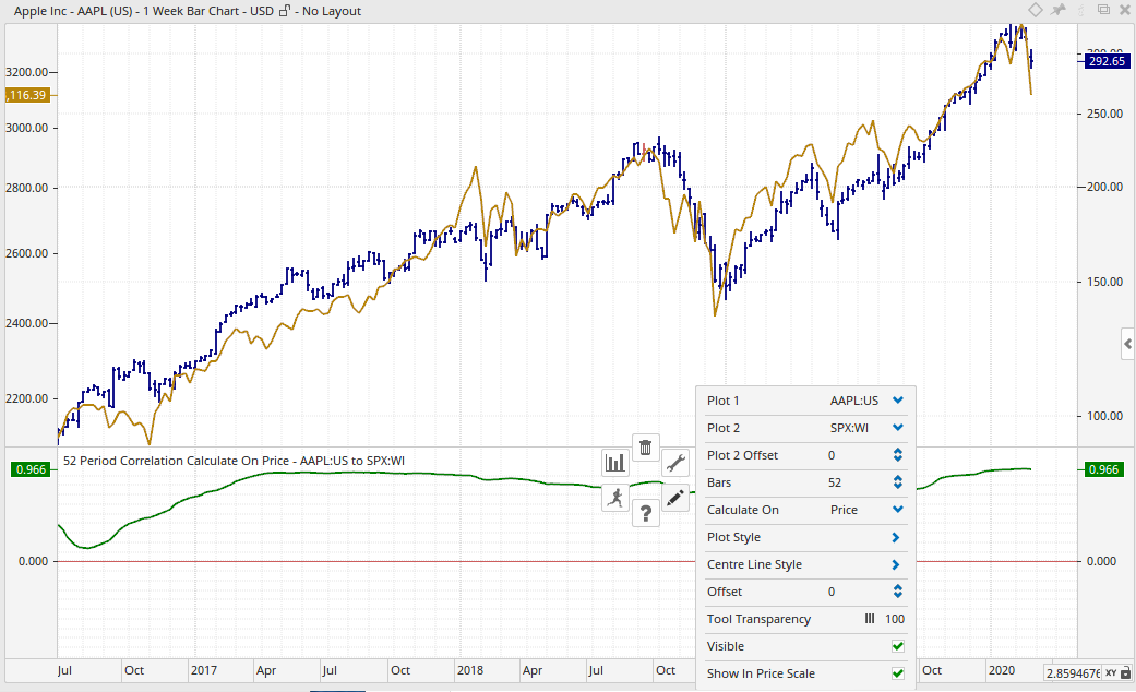
Using “% Change” I get a correlation of 0.779, using “Price” I get a correlation of 0.966.

Then I used the tool “Pearson’s Correlation Coefficient”. This tool has NOT the option to use “% Change”, it calculates only with absolute price changes. I think this is so.

correl#3

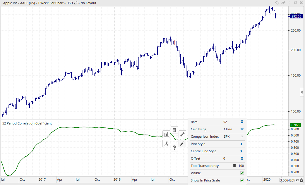
The correlation is 0.996, the same as using the tool “Correlation” and using “Price” in the setting “Calculate on”.

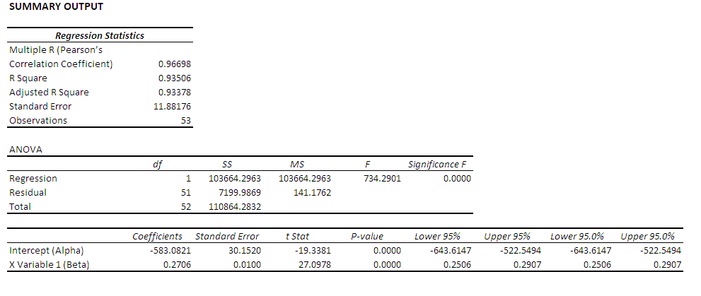
Now I created a script to calculate R-Squared.

correl#4

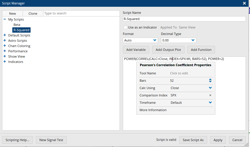
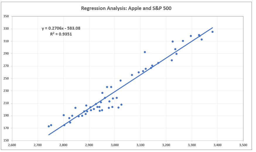
Then I created a chart to display R-Squared.

correl#5

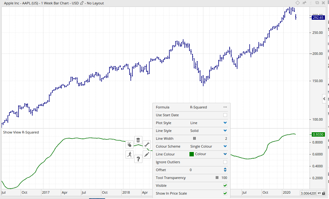
R-Squared is 0.933. That is of course correct since 0.966 * 0966 = 0.933. So far so good, no problem.

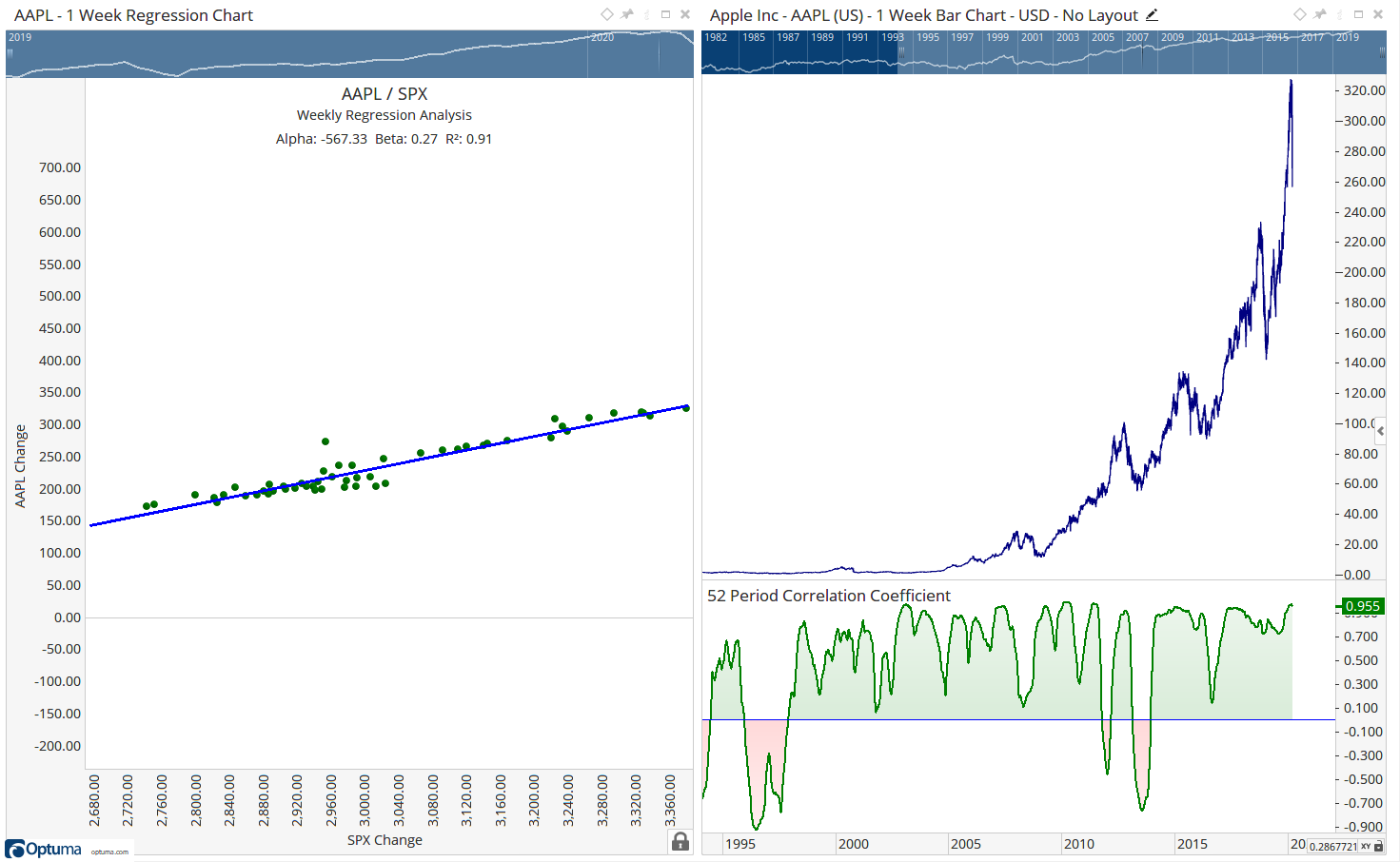
Then I used the tool “Regression Chart”.

correl#6

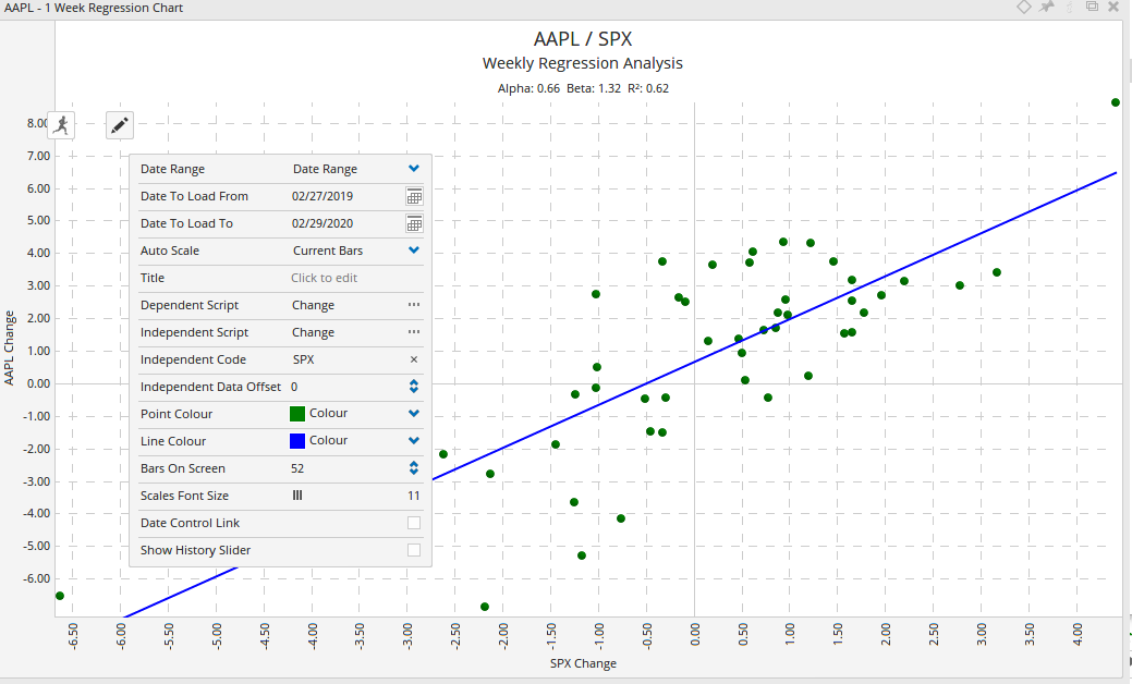
As you can see at the top of this chart R-Squared (R2) is 0.62!!!

Now the issue gets challenging. What is the right R-Squared number 0.62 or 0.933. Statistically this is a real big difference.

Using the tool “Correlation” and the setting “% change” in “Calculate on” I get a correlation of 0.779. Squaring 0.779 (0.779 * 0.779) and you get R-Squared of 0.61 very close to 0.62.

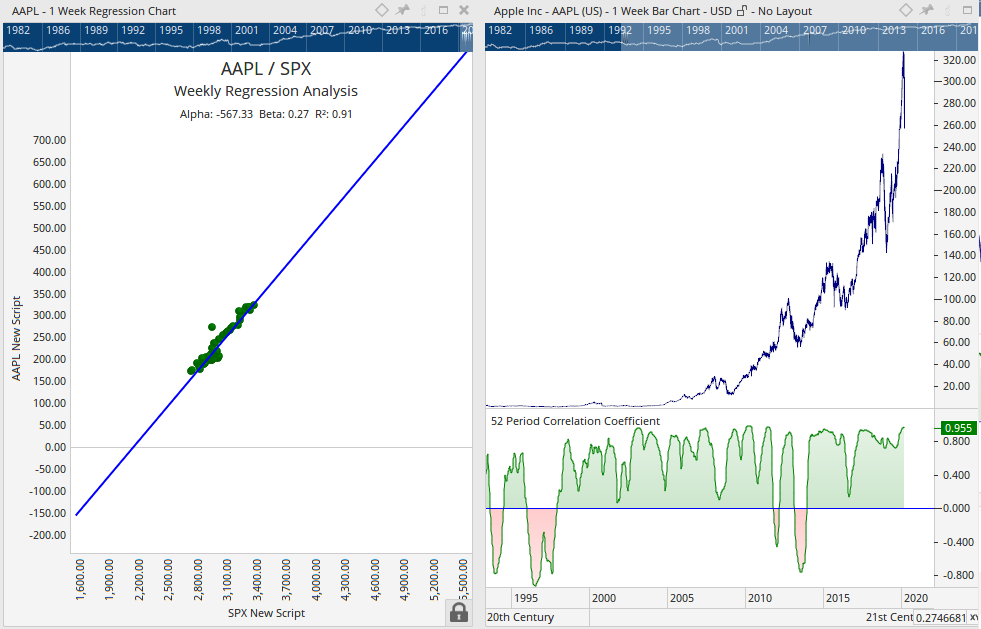
In the tool “Regression Analysis”, see screen shot above, the setting for the “Dependent Script” and for the “Independent Script” is “Change”. The script for “Change” is the following:

correl#7

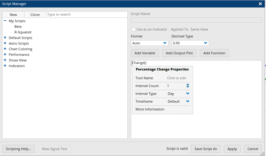
So now we have all the puzzles together and need only to understand what is going on.

  1. The tool "Correlation" allows the settings for "% Change" and "Price"
  2. The tool "Pearson's Correlation Coefficient" uses only "Price"
  3. The tool "Regression Analysis" has as standard setting "Change".
Now what is right, using "% Change" or "Price"?

As far as I understand the issue of regression analysis and correlation it is done using ONLY absolute price changes and not %-changes.

When regression analysis is usually done with price changes, why is in the tool “Regression Analysis” the standard setting “Change”?

What do you think is the “right” correlation, using %-change or absolute price change?

What script have I to use in the tool “Regression Analysis” to use absolute price changes and not %-changes?

I hope I have made the issue clear, a really very subtle issue.

Thanks

Thomas

Hi,

I made the same regression analysis in Excel using the “Data Analysis” add-in and using “Regression”.

Here is the statistical output from Excel:

And the Chart:

I have also attached the Excel file.

As you can clearly see, Excel uses absolute price change to calculate the regression analysis.

The Excel “Pearson’s Correlation Coefficient” (Multiple R) is: 0.96698, the same as in the Optuma tool “Pearson’s Correlation Coefficient” and in the tool “Correlation” using “Price” as setting in “Calculate on”.

The Excel R-Square is 0.93506, nearly the same as in Optuma. The really extreme small difference results form rounding, nothing to worry about.

I think it is know clear that using the absolute price change is the correct setting and not the %-change.

I would therefore recommend changing the standard setting “Change” in the tool “Regression Analysis” with a new standard script setting for absolute price change as used in the tool “Pearson’s Correlation Coefficient”.

Please inform me about the correct script to use in the tool “Regression Analysis” to calculate the absolute price change for the regression analysis.

Thanks

Thomas

Regression.xlsx (23.3 KB)

Since the level of prices violates stationarity, should we always use % change or difference in log prices for regressions?

Hi Thomas,

Sorry for the delay, I needed time to process this all. You are right that the Regression chart uses percent while the Correlation calculations use raw prices.

In the Regression Chart, just change the Dependent Script and the Independent Script to be “Close()” and it will match the square of the correlation. (See below). Also make sure that you change the correlation to only use Close - it uses HLC by default.

I am a little cautious of forcing people to use Price because regression functions assume stationarity (what Michael was suggesting). Our raw price data is not stationary (ie it trends over time) so we need to de-trend it. The easiest way is to use %change - and I believe that is the standard way in finance. Other ways are to use centered moving averages etc - this is what JM Hurst did in the 70’s before he applied his Fourier analysis.

The other issue is that when we use Price in a Regression analysis we a quantifying a per share value for excess returns. That is really hard to bring back into expectation. By doing the regression analysis in percent we now have a simple way of saying “If I fully invested in AAPL vs SPX, my returns (Alpha) would have been 66% better” Using your chart above. Put a Chart Element and set it to a script “CHANGE(INT_TYPE=Year)” to see this.

I also can not force percentage change as we may want to run the correlation functions over a data set which is stationary. Finally, I have to be very careful about changes as we have thousands of clients and we have no way of knowing if these tools are in their workbooks. If I force a change I can break the way that they are using the tools. This is why we add to tools but never “change” them.

All the best

Mathew


For the benefit of others reading this let me define a couple of things:

  • r is the symbol we give to correlation — more correctly Pearson's correlation. There are other calculations but this one is the most common. The range of values is -1 to 0 to 1.
  • r² is the Coefficient of Determination. Which ranges from 0 to 1.
The relationship should be simple. r² in the Regression chart should be the square of the Pearsons Correlation value. But the calculations have to be using the same data.

On the Regression Chart, Alpha is the excess returns over the benchmark. ie did we make more than the index. Beta is a volatility measure, High Beta stocks have a value that is over 1. In the chart below (which is in Price not %) it means that for a 1 point move in the SPX we expect a 27c move in Apple.

reg


Hi,

thank you Michael and Mathew for your replays. I too made some further “investigation” in this regression issue and agree with you both completely that it is better to use %-changes as a way to make regression analysis in finance.

As Mathew has pointed out the Alpha value makes no real sense when using absolute price changes. Only if we use %-changes to make the regression analysis the Alpha value makes sense.

But ones issue remains to be aware of is that the tool “Pearson’s Correlation Coefficient” uses only absolute price changes.

As we now have made clear, in finance it is better to use %-changes when doing regression analysis and so it is better to use the tools “Regression Analysis” and “Correlation” since both tools allow the setting “% change”. The tool “Pearson’s Correlation Coefficient” uses only absolute price changes, that we need to be aware of.

One final question to you Mathew regarding your regression chart. I have tried to recreate it. That was possible, no real problem. But one thin I was not able to recreate was the scaling of the x-axis in the regression chart.

How did you scaled the x-axis? In the regression chart tool there is only one setting for scaling that is “Auto Scale”. I set it to “Manual”. Doing so I was able to get the y-axis the same way as yours but my x-axis is completely different than yours.

regression

Thanks for your great assistance.

Thomas


Hi,

another issue about regression analysis.

I have created the following script to calculate R-Squared:

POWER(CORREL(CALC=Close, INDEX=SPX:WI, BARS=52), POWER=2)

This script is in some way wrong since the function “CORREL” is the function of the Pearson’s Correlation Coefficient. But the Pearson’s Correlation Coefficient uses absolute price changes.

To calculate R-Squared with %-changes the function “CORREL” can’t be used. We had to use the function “CRL” since this is the function for the tool “Correlation”. With this tool we can use %-changes.

I have tried the following script to calculate R-Squared using the function “CRL”:

POWER(CRL(CALCSTYLE=% Change, BARS=52), POWER=2)

The script gives the value “0”, so it is wrong. That is logical since we had to determine the two securities from which we want to calculate R-Squared.

We surly need to use the GETDATA() function but twice, for each of the two securities.

How do I incorporate two GETDATA() functions into the “CRL” function?

Or simple, what is the right script to calculate R-Squared using %-changes?

I hope this is the last post on this subtle topic from me.

Thanks

Thomas

Hi Thomas,

You can pass two variables into the CRL function.

Here is an example

d1 = Close();
d2 = GETDATA(CODE=SPX:WI);
CRL(d1, d2, BARS=52, CALCSTYLE=% Change)

Hope that helps

Mathew

Hi Mathew,

thank your very much for the replay on the weekend.

In my post above I wrote the following:

"One final question to you Mathew regarding your regression chart. I have tried to recreate it. That was possible, no real problem. But one thin I was not able to recreate was the scaling of the x-axis in the regression chart.

How did you scaled the x-axis? In the regression chart tool there is only one setting for scaling that is “Auto Scale”. I set it to “Manual”. Doing so I was able to get the y-axis the same way as yours but my x-axis is completely different than yours."

Can you give me a tip how to scale the x-axis in the regression chart?

I have seen a regression chart from Darren on twitter (https://twitter.com/Optuma/status/1233644950954233856/photo/1) he too has “mastered” to adjust the x-axis.

I was able to scale the y-axis of the Apple/S&P 500 regression analysis the same way Darren did but not the x-axis.

Where is the trick?

Thanks

Thomas

Hi,

for those interested in the subject of regression analysis in finance, the correct script to calculate R-Squared using %-change - as it is usually used in finance - is:

d1 = Close();
d2 = GETDATA(CODE=S P 500:MUFD);
POWER(CRL(d1, d2, BARS=52, CALCSTYLE=% Change), POWER=2)

This scripts calculates R-Squared with the stock in the main chart window and the S&P 500 with a period of 52 weeks.

The script above from Mathew calculates the correlation coefficient using %-change. If you square the correlation coefficient you get R-Squared. The correlation coefficient is also called the “Pearson’s Correlation Coefficient”.

But as already mentioned above, in Optuma the tool “Pearson’s Correlation Coefficient” uses price changes and not %-changes.

Only the tool “Correlation” (CRL) allows the setting %-change to calculate the correlation coefficient.

Thanks

Thomas


Hi Thomas,

Re the scaling of the chart. I usually just adjust the size of the actual chart. I also leave it on auto. (that tweet was me).

One thing which I have wanted to do is lock it down more so that a Beta of 1 was exactly 45 degrees. The concern with scaling is that you can not see the relationship at a glance. Unfortunately this never gets high enough in my todo list to get looked at.

All the best

Mathew

Hi,

I have further question to the script to calculate R-Squared.

The script is the following:

d1 = Close();
d2 = GETDATA(CODE=S P 500:MUFD);
POWER(CRL(d1, d2, BARS=52, CALCSTYLE=% Change), POWER=2)

It works fine (see above). As you can see in the script it uses 52 Bars.

Does that mean if I use a daily chart it calculates R-Squared for 52 days?

If I have a “1 Day” watch list and use the above script in the “1 Day” watch list does that mean it calculates R-Squared for 52 days?

On the other hand is it necessary to set the setting to “BARS=252” to calculate in a “1 Day” watch list R-Squared for 1 year?

Thanks

Thomas

Hi Thomas,

You’re right, 52 Bars would be 52 Days on a Daily chart or 52 Years on a Yearly chart.

252 is the number to use for yearly - it’s what we use in volatility calculations when going from yearly to daily volatility.

The issue with daily correlation is that you are now measuring 252 results in each. While two securities can move together every day, it is rare as daily noise hides the correlation. Weekly (52 samples) is better as it allows us to see that in general the two move together.

All the best

Mathew

Hi,

for those interested in this topic Mathew has updated all correlation and regression calculations. With version 1.6 we are able to use the option to make the calculations with the LN function (natural logarithm) e.g. LN(Close/Close[1]) instead of simple price %-change calculation e.g. (Close/Close[1])*100.

See the post “Beta #2” (https://forum.optuma.com/topic/beta-2/). All confusing calculation results are now no longer present.

Thomas